PID Controller Design using Simulink MATLAB: Tutorial 3

In this tutorial, we will discuss the workings of a simple PID (Proportional Integral Derivative) controller. Then we will see how to design it using MATLAB’s Simulink tool. At the start, we provide a brief and comprehensive introduction to a PID controller. Then we will look at a simple block diagram that can help us implement a PID controller on our own. After that, we will provide an example of a controller using Simulink. We can design a PID controller in two different ways; we will implement both of these, and after the implementation, we will compare the results from both methods. At the end, a simple exercise is provided regarding the concepts and blocks used in this tutorial.

You may also like to check out the following tutorials on Simulink: Getting started with Simulink and Solving differential equations in Simulink 

Introduction to PID Controller

PID controllers find their applications in industrial settings because of their ease of use and satisfaction with performance. They are capable of providing the user with access to a large number of processes. The cost/benefit ratio of these controllers is way higher than any other controller. There are many techniques for their design because of their widespread use for tuning the parameters of PID, i.e., Kp, Ki, and Kd. Hence, these parameters improve the performance of the implementation of additional functionalities in a PID controller.

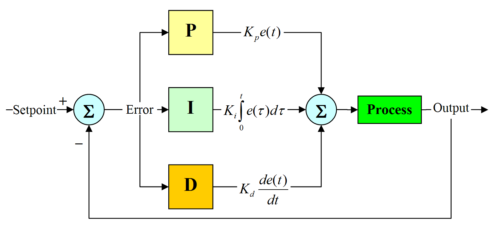
Nowadays, the use of control loops is almost everywhere. Anytime we adjust our current work according to the results obtained from previous work, we form a control loop. For example, when we feel cold and turn our heater on, we form a feedback loop, and when we press the accelerator of a car whenever we are getting late, we again form a control loop. Whenever we make any change in the environment by sensing the previous results of that process, we form a close control loop in our mind. Changing the speed of the car is one of the best examples. The block diagram of a simple PID controller is provided in the figure below.

PID controller Design using Simulink

In this section, we will see how to design a PID controller in Simulink. But first, we will move towards a simple example regarding the working of a simple PID controller using Simulink. In Simulink, a PID controller can be designed using two different methods. Simulink contains a block named PID in its library browser. We can implement the PID controller by either using the built-in PID block or by designing our own PID controller using the block diagram. The results of both of them are, however, not the same, as we will see shortly.

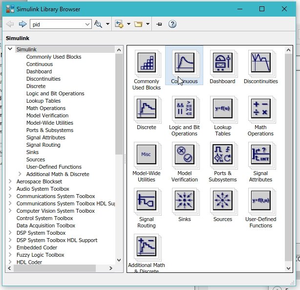
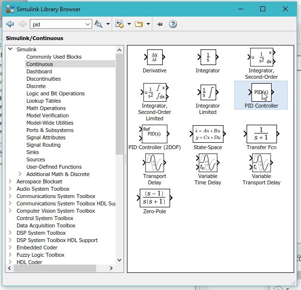
Let’s now begin with the programming part. Open MATLAB and then Simulink, as we did in the previous tutorials. After that, open the library browser, and from the library browser, select the continuous subsection as shown in the figure below.

Placing Components

Double-click on the continuous block in the library browser, and from that block, select the PID block. Refer to the figure below.

Sources

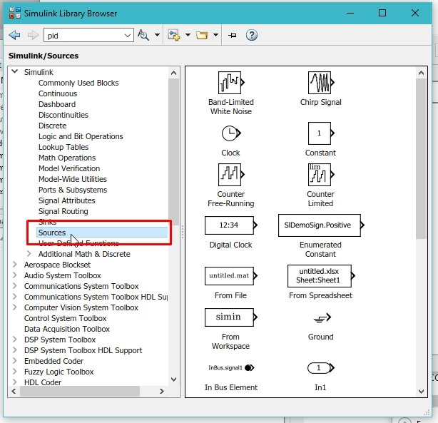
This block is a PID controller itself. The next thing we need is a supply, i.e., a step response, to apply to the PID. Now, from the Simulink Library Browser, select the sources as shown in the figure below.

Step Response

From the sources subsection, select the Step block, which we will use as an input source for the PID block. Refer to the figure below.

Sink

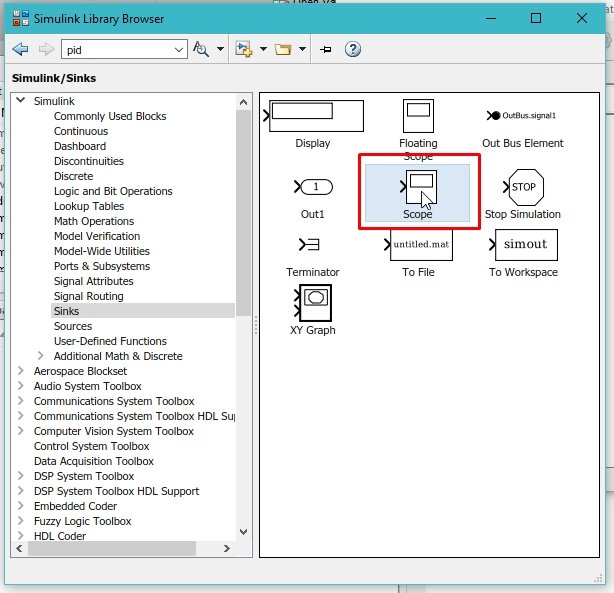
Now click on the Sinks subsection from the list at the left of the library browser. As we can see in the following figure.

Scope

From the sinks subsection, select the scope to display the output. We can also access the scope block from the commonly used blocks section in the library browser. The second way is to search the block by typing its name in the search bar of the library browser. Refer to the figure below to see the scope block selected from the sinks section.

Transfer Function

We also need a system to apply the PID controller to it. By placing a system here, what we actually mean is to place a transfer function of the system in the block diagram. We can get a transfer function block from the continuous section of the library browser in Simulink. Refer to the figure below.

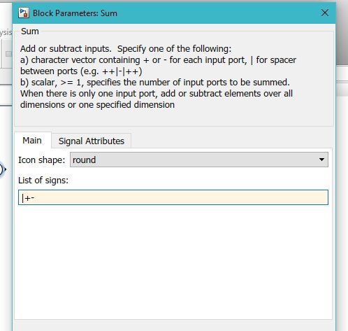
Sum Block

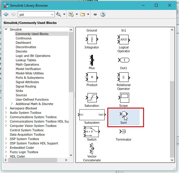
The last block we will place is the sum block to subtract the feedback path of the close loop system. The sum block can be obtained from the commonly used blocks, as shown in the figure below.

The components placed so far are shown in the figure below.

What we need to do is change the parameters and properties of all the blocks according to our requirements. For instance, let’s first change the list of signs in the summation block, as we need the second sign to be negative to subtract the feedback path from the current input. Refer to the figure below.

Setting Parameters

Now we need to update the transfer function according to our needs. Double-click on the transfer function block and change the values of the numerator and denominator as shown in the figure below.

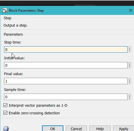
Double-click on the step response block and adjust the properties as shown in the figure below. We did this to start the step at 0s.

Now double-click on the PID block and change the values of Kp, Ki, and Kd as shown in the figure below.

Simulink Model 1

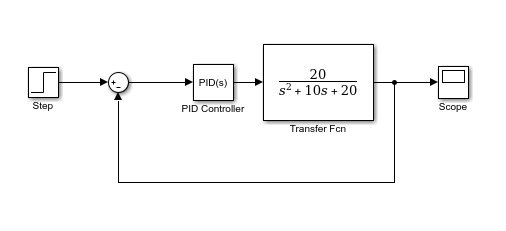
These are just tips to improve the output results. We can update them later for the tuning purposes of PID. Connect all the blocks with wires, and the complete circuit diagram will look like the one shown in the figure below.

Model Configuration

The only step left is to update the model configuration according to the step response and adjust the sampling time of the system. Click on the model configuration icon, as shown in the figure below.

In the model configuration dialog box, change the variable step to fixed steps and change the sampling time to 0.01 s, as shown in the figure below.

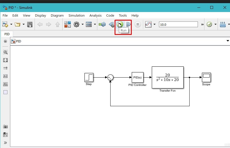
These properties have a great impact on the response of the system. Now run the system from the run icon at the top of the Simulink page, as shown in the figure below.

Simulation of Model 1

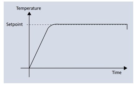
After running Simulink’s simulation, open the scope to see the generated waveform. The output of the waveform is shown in the figure below.

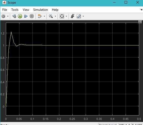
The output is a little overdamped, but we can adjust it by tuning the values of Kp, Ki, and Kd.

Let’s now move toward the second method to implement the PID controller in Simulink. Place three gain blocks in a row, and at the input, connect the output of the step block and name them Kp, Ki, and Kd. Refer to the figure below.

At the output of the Ki block, place an integral block as we have previously. And from the continuous section of the library browser, select the derivative block as shown in the figure below.

Place this block at the output of the Kd gain block and sum up all these gains using a sum block, as shown in the figure below.

Simulink Model 2

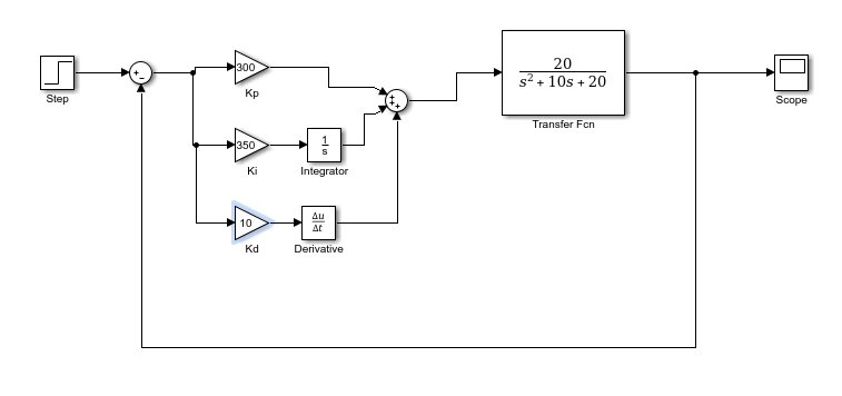
Adjust the values of the gain as we did in the previous method, and the complete block diagram of the PID controller is shown in the figure below.

Simulation of Model 2

Run the block diagram again and open the scope to see the response of the system, as shown in the figure below.

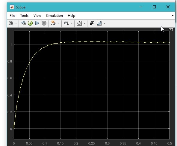
The output is slightly underdamped, but we can adjust it by tuning the gains of the PID controller. We leave it as an exercise for the reader.

Exercise

• Tune the values of Kp, Ki, and Kd to make the step response of the transfer function critically damped.

Conclusion

In conclusion, this tutorial provides an in-depth overview of PID controllers using Simulink. It covers step-by-step procedures along with an explanation of an example to help us better understand the concept. You can utilize this to design more complex designs for the PID controller. At last, we have provided an exercise to reinforce the concept of this tutorial. Hopefully, this was helpful in expanding your knowledge of designing and simulating PID controllers using Simulink.

You may also like to read:

• N76E003AT20 Microcontroller Unit
• Interrupt Processing ARM Cortex-M Microcontrollers
• Pulse width measurement using pic microcontroller
• ATtiny2313 8-bit AVR Microcontroller
• BeagleBone Black Pinout, Pin Configuration and Features
• ESP32 Bluetooth Low Energy (BLE) using Arduino IDE

This concludes today’s article. If you face any issues or difficulties, let us know in the comment section below.