In this tutorial, we will look at a brief and concise introduction to MATLAB and one of its tools, known as Simulink. This is an introductory tutorial, and here we will explain the very basics of MATLAB as well as Simulink. Introduction to some of the basic functions and libraries of Simulink, and with the help of explanation, we will perform a simple example and discuss its results. At the end, a simple exercise is provided for you to do on your own. In the upcoming tutorials, we will expect that you have done that exercise.
Introduction to MATLAB
MATLAB is a multi-purpose numerical analysis environment. It is a high-performance fourth-generation programming language that finds its applications in technical computing. It is a multi-purpose programming environment, and we can use it for various problems like developing algorithms, matrix calculation, running algorithms, data visualization, and making an easy-to-use graphical or simple user interface (UI).
Drawing graphs, either 2-dimensional or 3-dimensional, is no longer a difficult task when you have MATLAB to perform it. Also, it is freely available for students on the website of MathWorks for those who have an interest in learning in a highly diverse programming environment.
Introduction to Simulink
Out of the magnificent number of tools in MATLAB, Simulink is one of the most widely used and high-performance tools. As it is one of the tools of MATLAB, it cannot be compared with MATLAB. MATLAB is the main application that MathWorks provides, and Simulink is a graphical programming environment that allows us to simulate, design, and execute a program in the form of blocks.
For instance, there is a block of summation present in the libraries of Simulink, and there is a block of a constant as well as input, which can help us provide the input to that summation box. There is also a block of output and an oscilloscope to display the output of the summation block. This is just a very simple example, but it provides us with a wide range of components, which we will discuss further after some time. Throughout this session, we will be using a number of components to remove any ambiguity about this software.
Getting Started with Simulink
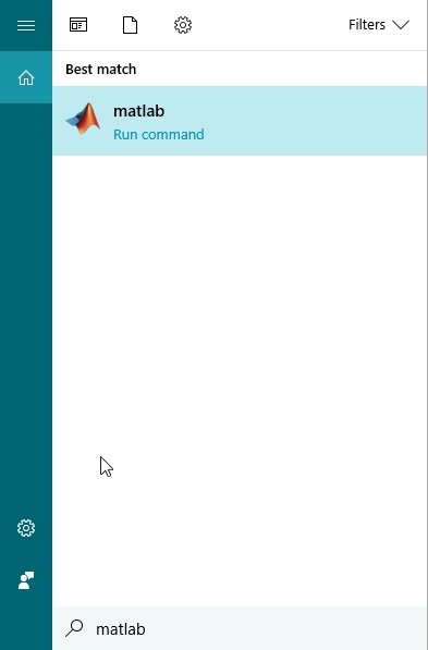
To start with this tutorial, let’s first open MATLAB and then Simulink. In the search bar of the system, type “matlab” (if installation is present on the computer). We will see the icon pop up as shown in the figure below.
It takes some time to open this program, and after opening, the following window will appear as shown in the figure below.
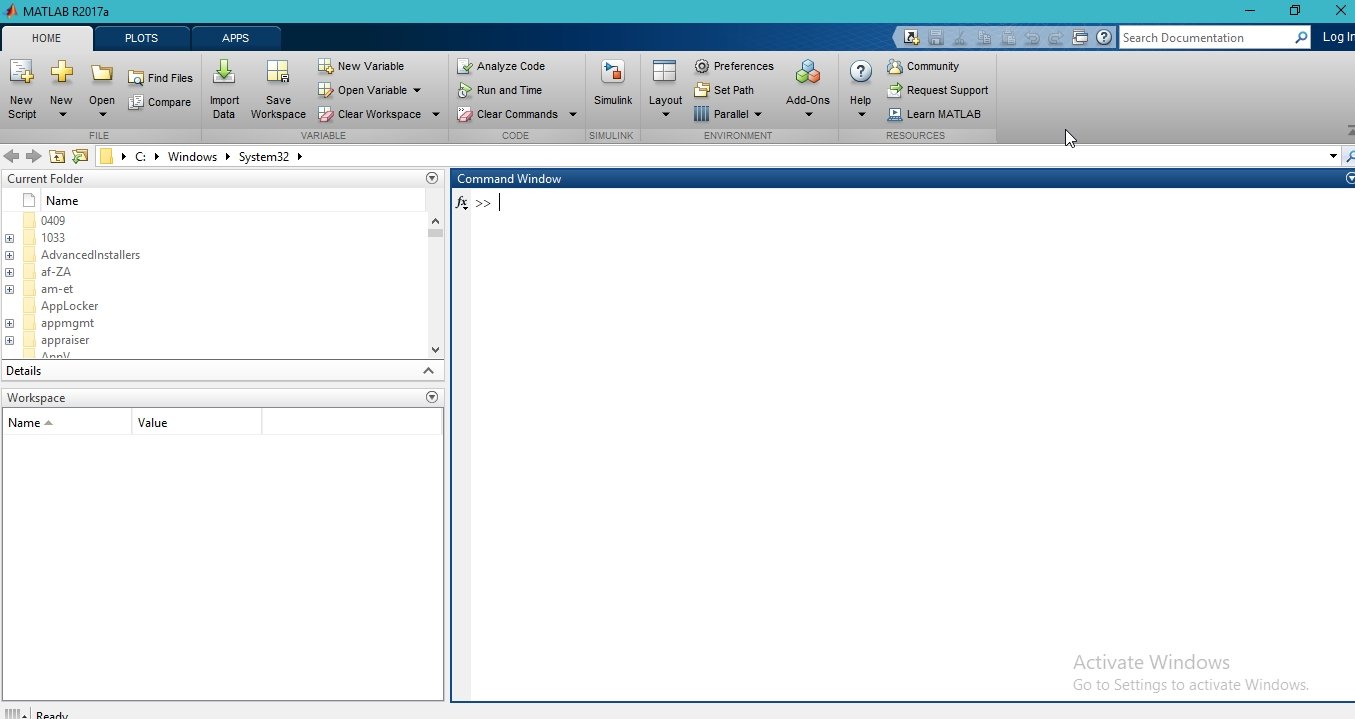
Opening Simulink
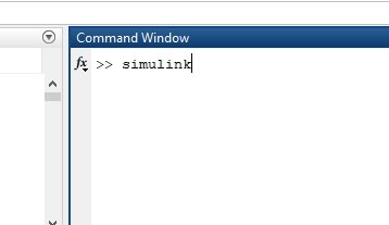
Now, the next step is to open Simulink. We can open it by writing “Simulink” in the command window of MATLAB, similar to the figure below.
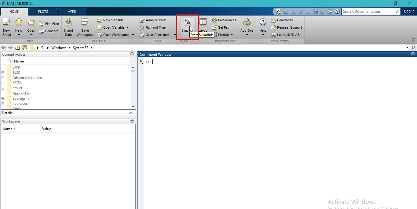
Another way to open it is by using the icon present at the top of the home panel of MATLAB, as we can see in the following figure.
Opening Simulink also takes quite a lot of time because it is heavy software. Once Simulink is open, it will show a start page, as we can see in the following figure.
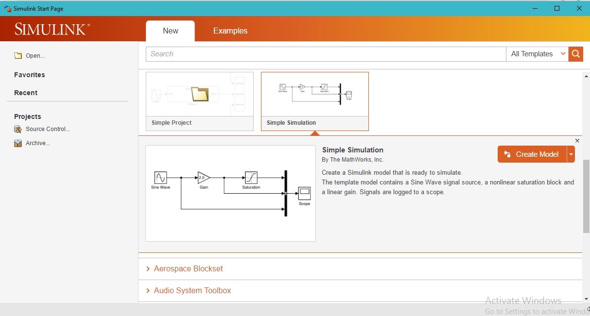
Simulink Examples
There are also a number of built-in examples in it. So that we can run them and learn about the workings of the different blocks present in Simulink. We can access them from the window at the top of the Simulink starting page. Refer to the figure below.

These examples can be used as a head start to understanding the workings of Simulink as a beginner before directly jumping into the programming environment of Simulink. We will leave exploring these examples as an exercise for the students. Now let’s create a new project and start working with Simulink. Click on blank project on the start page of Simulink. Refer to the figure below.
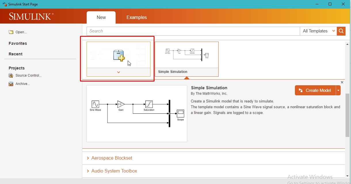
This will create a new blank project, as we can see in the following figure.

This is an unsaved project, and the changes we make to it will go to waste. Therefore, first of all, we will save this project so that we can access it sometime later. Click on the file button and then click on “save as“, as shown in the figure below.
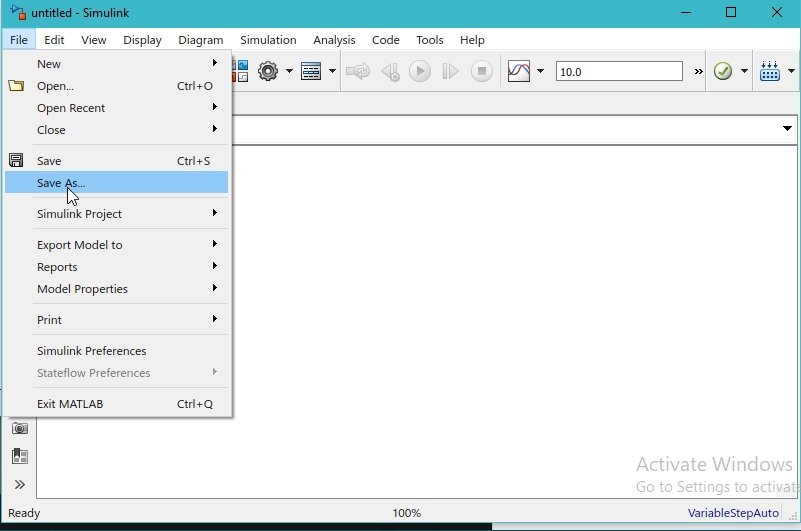
Library Browser
After saving the project in the directory of our choice, the next thing we will like to look at is the browsing library of Simulink. We can access the Library Browser by clicking on the VIEW button at the top of the list next to the file and then clicking on the library browser, as shown in the figure below.

Another way to access the library browser is by clicking on the library browser icon. Refer to the figure below.
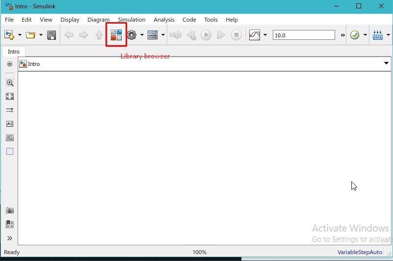
The library browser window will open up after clicking on this icon. This window is shown in the figure below.
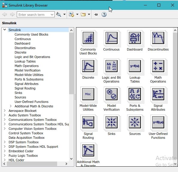
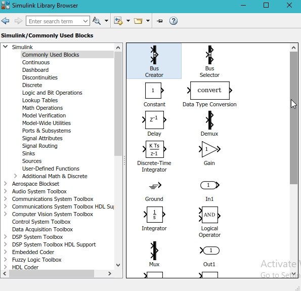
This window contains almost all the blocks one can need to write a program, starting from a simple multiplication problem to the working of a motorcycle in the robotics section. The most commonly used blocks in Simulink are available in the Commonly Used Blocks subsection. Double-click on the subsection to have a look at the blocks, as shown in the figure below.
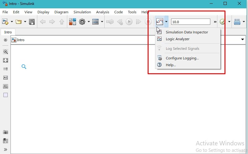
On the top bar of Simulink, there is an icon to provide a logic analyzer. As the name suggests, it is used to analyze the output of the block diagram system. Refer to the figure below to see the location of the logic analyzer in the Simulink window.
Making First Block Diagram with Simulink
Let’s do a simple example to understand the workings of Simulink in a little more depth. Here, we will perform a simple AND operation and run the program. From the commonly used blocks, select the AND operator and also a Scope, which will act like an oscilloscope to analyze the output of the operation as shown in the figure below.

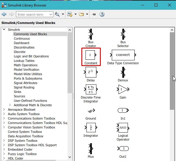
From the same library browser block, i.e., commonly used blocks, select a constant and place it at the input of the logical operator as shown in the figure below.
Placing Components
Place all the components as shown in the figure below.

Simulink Model
When we hover over the arrow head of each of the blocks, the pointer will convert to a simple cross and allow us to start the connection of the wire. Connect the constants at the input of the logical operator, and at the output of the logical operator, connect the scope. Now run the program using the run button, as shown in the figure below.

Simulation
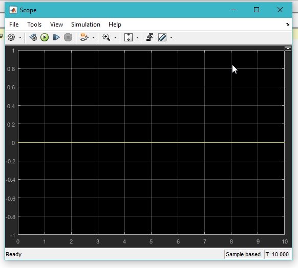
After running the program, double-click on the scope, and a window will appear showing the output of the operator in the form of a wave on the oscilloscope. Refer to the figure below.
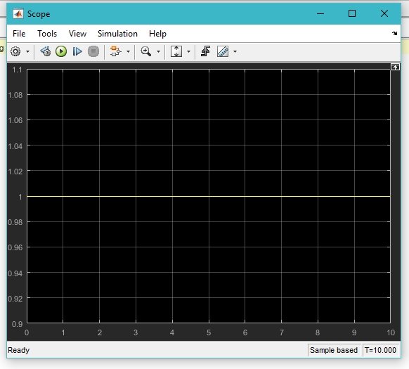
Now we will test the program with different input values, i.e., 1 and 0. The output will change in accordance with the theory. It turns to 0 and shows expected results, as shown in the figure below.
Exercise
- Explore some of the built-in examples of Simulink and try learning the workings of the different blocks used in the featured examples.
Conclusion
In conclusion, this tutorial provides an in-depth overview of how to get started with the MATLAB Simulink Tool. It covers step-by-step procedures along with examples and their explanation to help us better understand the concept. You can utilize this concept to write and develop a program in the MATLAB Simulink tool. At last, we have provided an exercise to reinforce the concept. Hopefully, this tutorial was helpful in expanding your knowledge in regards to Simulink.
You may also like to read:
- Simulation and design of Three phase Rectifier in Simulink MATLAB
- ESP32 ESP-NOW Getting Started Tutorial with Arduino IDE
- Calculate Factorial of a Number in LabView: Tutorial 35
- STM32 I2C Communication Guide – HAL Code Examples Slave & Master – DMA Interrupt
- MPU6050 Sensor Module Interfacing with Pic Microcontroller
- DC Motor Control with LabVIEW and Arduino – Tutorial 3
This concludes today’s article. If you face any issues or difficulties, let us know in the comment section below.


wonderful