Quadratic root calculation in LabView : tutorial 26

In this tutorial, we will learn how to calculate the roots of a quadratic equation using LabView. Quadratic root calculation is one of the easiest but most hectic tasks, in our opinion. In this tutorial, we will try to design a VI that takes the coefficients of a quadratic equation as inputs. After processing, it will display the roots of the equation at the output. At the end of the tutorial, we have provided an exercise for you to do on your own, and in the next tutorials, we will assume that you have done those exercises and not explain the concept regarding them.

Quadratic Equation

Here we will explain the quadratic equations and the simple approach that is used to solve them. A quadratic equation is a fundamental mathematical expression of the form ax² + bx + c = 0. The roots of a quadratic equation are the values of “x”, whereas a, b, and c are constants that satisfy the equation, making the expression equal to zero. To calculate these roots, we often use a simple process that includes employing the quadratic formula: x = (-b ± √(b² – 4ac)) / 2a. This formula enables us to determine the roots as real and complex, providing insight into the behavior of the quadratic equation. This straightforward yet crucial procedure forms the basis of solving quadratic equations, underpinning numerous applications in mathematics, science, engineering, and beyond.

In the next section, we will see how we can implement this formula in LabVIEW to get the roots of a quadratic equation with the help of coefficients.

LabVIEW Example: Quadratic Root Calculation

We will now design a VI that takes the three coefficients of a quadratic equation as an input. It will return the roots of the equation as output. Create a VI as I have explained in Tutorial 1, and save it for future use. On the front panel, press right-click, and from the Control Palette, select Numeric, and then select Control, as shown in the figure below.

Figure 1: Numeric control placement

Place three similar indicators and name them a, b, and c. This is because a simple quadratic equation has only three coefficients. See the figure below,

Figure 2: Input controls

Indicator Placement

Now from the Control Palette on the front panel, select Numeric. After this, select the Indicator as shown in the figure below.

Figure 3: Numeric indicator placement

Place two indicators of type numeric and name them x1 and x2 because a quadratic equation has only two roots. Refer to the figure below.

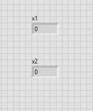
Figure 4: Output indicator

Nodes Placement

LabView has a structure named formula node, in which we can write code in MathScript. On the Function Block, press right-click, and from the Function palette, select Structures. At last, select the formula node, as shown in the figure below.

Figure 5: Formula node placement

Place the block in between the input controls and the output indicators. Right-click on the left side of the formula node, i.e., on the input side, and from the dropdown, select Add input, as shown in the figure below.

Figure 6: Adding input node

Similarly, on the right side of the formula node, i.e., on the output side of the node. Press right-click and from the dropdown menu select Add output, as shown in the figure below.

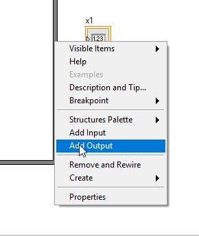
Figure 7: Adding output node

On the input side, create three nodes because of the three input co-efficients, and on the output side, create two nodes as we have two roots as the output, as shown in the figure below.

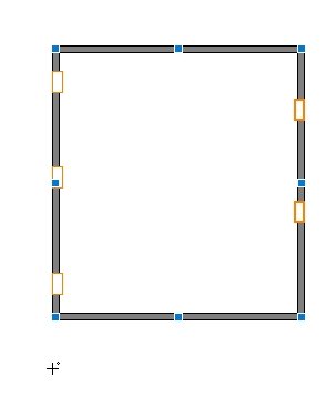
Figure 8: Inputs and outputs

Connection Diagram

Connect the input nodes to the input controls and the output nodes to the output indicators and name the variables, as shown in the figure below.

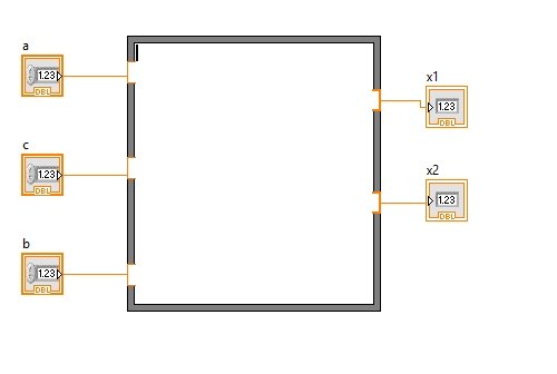
Figure 9: Connections

Don’t forget to align each group of blocks according to the orientation, as we have done here and already explained in previous tutorials.

Now inside the formula node, write a MathScript code to calculate the roots of a quadratic equation i.e. As shown in the figure below,

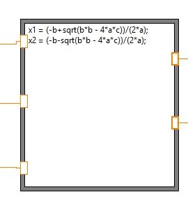
Figure 10: Formula code

If you are not familiar with any of the command in LabView simple open the built in help window of LabView see the detailed description of the command or block about which you want to know.

The nodes you created on the input and output side of the formula node will store the value of the controls you connected to them or for the output case they will display the value from the formula node to the output indicator.

But, where will it store the value from the input control?? We have to name the node with a specific variable in which it will store the value from the input control and will use that dummy variable inside the formula node.

Similar is the case with the output nodes, all the values assigned to any dummy variable inside the formula node i.e. x1 and x2 in our case will have one output node assigned to it.

No of output nodes must be equal to the number of assignment operator used inside the formula node and we have to name output nodes too according to the dummy variable inside the formula node as shown in the figure below,

Figure 11: Naming of the node.

Output

Lastly, on the front panel give specific input values to the input controls you created in the start and run the VI. Thus, the output indicators will display the roots of the equation formed by using the input variables as shown in the figure below,

Figure 12: Output of the VI

The VI we designed here will calculate only the real roots of the quadratic equation

Exercise

Use your knowledge and try to generalize the above VI for finding imaginary roots too.

Conclusion

In conclusion, this article provides an in-depth overview of how to calculate quadratic roots with the help of VI in LabVIEW. This helps the user with a step-by-step procedure to design the VI that takes input coefficients and provides quadratic roots as output. All of this is explained with the help of figures for each case. You can utilize these concepts for working with quadratic roots to solve complex math problems using LabVIEW. Lastly, we have provided an example to reinforce the concept of solving quadratic equation-related problems using VI. We hope that this tutorial has been helpful in expanding your knowledge of LabVIEW.

Quadratic Root Calculation in LabVIEW: Tutorial 26

Quadratic Equation