Data Flow in LabVIEW: Tutorial 20

In this tutorial, we will learn about the data flow of LabView. One might be wondering what dataflow is. Data flow is the flow of data during runtime. How does the execution of the block diagram occur when we run the VI, i.e., what is the order of execution? Is it from left to right or top to bottom (as in text-based programming languages)? At the start, we try to explain the data flow in LabView. After that, we design a VI, which will help us explain data flow in detail. At the end of the tutorial, we have provided an exercise for you to do on your own, and in the next tutorials, we will assume that you have done those exercises, and we will not explain the concept regarding them.

Introduction to Data Flow in LabVIEW

In computer science, the term data flow is extensively used and is based on the idea of disconnecting computational actors into stages that can execute concurrently. Streaming process is another term that can be used concurrently with data flow.

Data flow, or streaming process languages, have been subdivided into several forms. We can also define the architecture of the hardware of dataflow as an alternative to Von Neumann’s architecture. Reactive programming with spreadsheets is the most obvious example of data-flow programming. The values entered by a user are instantly transmitted to the next logical variable or formula for calculation.

In LabView, dataflow is considered one of the most important terms. A node present in a block diagram will execute only when data is present at all of its inputs, as you will see later in this tutorial. After the execution of a node, the output data of the node is transmitted to the next node in the dataflow path. The execution order of the VIs and functions on the block diagram is determined by the movement of data through the nodes.

Examples of Data Flow in LabView

We will now design a simple block diagram and try to explain the data flow through each node with its help. Let’s first design a single-node block diagram that will increment the input value by one. From the Function Palette, select Numeric and then select Increment, as shown in the figure below.

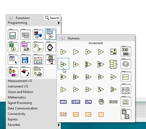
Block Diagram

Create a control at the input of this increment and an indicator at the output side, as shown in the figure below.

Turn on the highlight by clicking on the highlight button (with a bulb symbol on it), as shown in the figure.

Enabling this button will allow us to see the flow of data through the wires in the respective block diagram and easily view the execution flow of VI. Now, run the program using the run button orb by pressing <Ctrl+R> and see the flow of the data.

Data Flow

The nodes or wires in which data is not flowing yet will be grayed out, whereas the wires and blocks where data is flowing currently will be the color of the data type that is flowing, as is obvious in the figure below.

Obviously, the data will always flow from the input side to the output side. The output of the above block diagram present on the front panel is shown in the figure below.

2^nd Increment Block Diagram

Now, if we insert a node in the above block diagram, i.e., add an increment block, connect the input side of the second increment block to the output of the first, and at the output of the second block, create an indicator and give it a proper name, refer to the figure below.

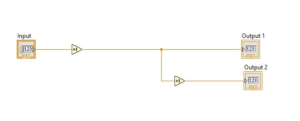
Now, if we run this block diagram with highlight ON, we will exactly understand the flow of data through a node.

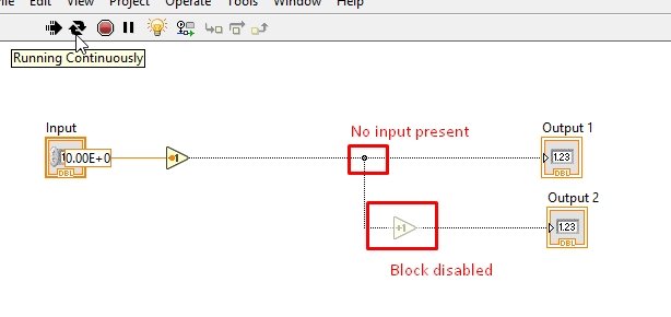
We can see in the above block diagram that the data coming from the input side increments by 1 first before reaching the second increment block.

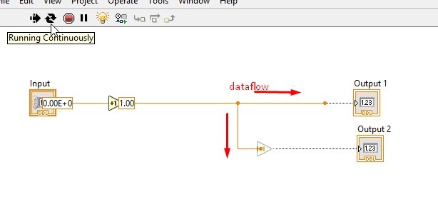
The second block is grayed out because it is currently disabled. LabVIEW VI enables this block only when all the inputs at the node are available. The data flowing from the upper wire, when provided to the node, will enable the node and hence the increment block, as shown in the figure below.

3^rd Increment Block Diagram

The same will happen when we add multiple nodes in the block diagram, i.e., if we insert a third node after the second increment block, as shown in the figure below.

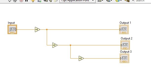
Data will start flowing from the input control, and at that time the VI will disable both nodes, as shown in the figure below.

Enabling Node

After that, when the data reaches the first node, it enables the second increment block because LabVIEW knows about the input to be present at the node. Refer to the figure below.

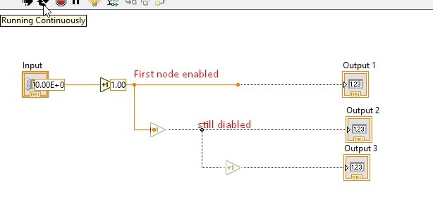
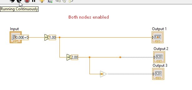
The above diagram shows that the flow has reached the first node and hence enabled the 2^nd increment, but the data isn’t yet present at the second node, so the 3^rd increment block is still disabled. The 3^rd block will be enabled only when the data reaches the 2^nd node and input is present at the node, as shown in the figure below.

This is the execution flow of the code in one block diagram, but what happens when multiple blocks not connected to each other run simultaneously? Which one of all the blocks will VI execute first?

Let’s discuss this with the help of an example. In the above block diagram, add another simple incrementing block with a control and an indicator and give some value to the control, let’s say 5, as shown in the figure below.

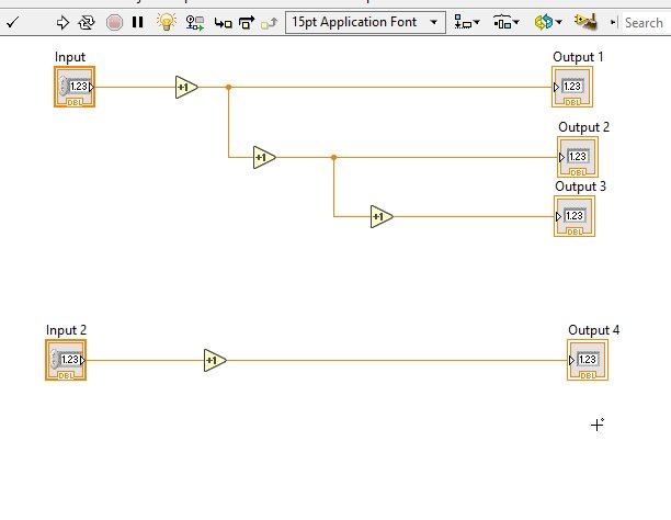
Multi-block data flow

When we run this program with the highlight button turned on, we can easily see the flow of the data, as shown in the figure below.

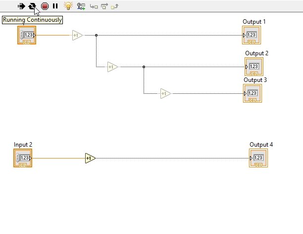
It is obvious from the above block diagram that the data flow in both block diagrams is parallel. The VI does not execute blocks at the same time in a complete VI; the discussion on this concept is in the sequence structure tutorial. If we want to execute one portion of code after another, we must create a node in between them, as we have done above in the 3-stage increment block.

Exercise

• Try to do the example we did in the previous tutorial (the one with the loop completion pop-p message) without using sequence structure, i.e., with the help of dataflow, managing the nodes method we discussed above.

(Hint: Use Boolean true and false blocks with a stop button)

Conclusion

In conclusion, this tutorial provided a comprehensive overview of data flow in LabVIEW. The tutorial began by explaining the concept of data flow and its importance in LabVIEW. It then proceeded to demonstrate examples of data flow through different block diagrams, highlighting how data is transmitted from one node to another. The tutorial also showcased the enabling and disabling of nodes based on the presence of data. Furthermore, it discussed the parallel execution of multiple block diagrams and emphasized the need for nodes to control the sequential execution of code. Overall, this tutorial served as a valuable resource for understanding and working with data flow in LabVIEW.

You may also like to read:

• SEPIC Converter Proteus Simulation
• ESP32 with MPU6050 Accelerometer, Gyroscope, and Temperature Sensor ( Arduino IDE)
• I2C LCD with STM32 Blue Pill using STM32CubeIDE
• Difference Between Raspberry Pi and Arduino
• Control Relay Module Remotely with ESP32 Web Server and 220V Lamp

This concludes today’s article. If you face any issues or difficulties, let us know in the comment section below.

<<Previous tutorial                                                      Next tutorial>>