Solving Differential Equations with Simulink: Tutorial 2

In this tutorial, we will explain the workings of differential equations and how to solve them using Simulink. At the start, we will provide a brief and comprehensive introduction to differential equations, along with some small talk about solving the differential equations. After that, we will provide a brief introduction and discuss the use of the integral block present in the Simulink library browser. Then we will discuss how it can help solve the differential equation. Lastly, we will solve an example of a second-order differential equation using Simulink, along with a description of each step and the use and working of each block. At the end, a simple exercise is provided regarding the concepts and blocks used in this tutorial.

How to Solve Differential Equations in Simulink 

In the Simulink library browser, there is a block with the name Integral. Refer to the figure below.

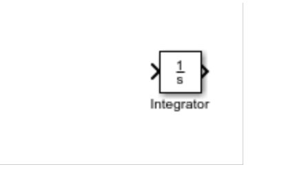
As the name suggests, this block calculates the integral of the signal we provide at its input, i.e., the left side of the block. In the case of solving a differential equation, the major thing we have to do is integrate the given equation, which will return the function without the derivative.

The integration of the function’s derivative is equal to the function itself. Here, the purpose of the integral block is the same. The number of integral blocks in a block diagram is equal to the order of the differential equation we are going to solve in the problem. For instance, if we want to solve a 1^st order differential equation, we will need 1 integral block, and if the equation is a 2^nd order differential equation, we will need 2 integral blocks. Let’s now do a simple example using Simulink in which we will solve a second-order differential equation.

Simulink Block Diagram of Differential Equation

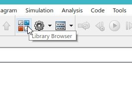
First, open MATLAB to start working with Simulink, as we did in the previous tutorial. Open Simulink by either typing simulink in the command window or using the Simulink icon. On the Simulink start page, click on the library browser icon to open the library browser. Refer to the figure below.

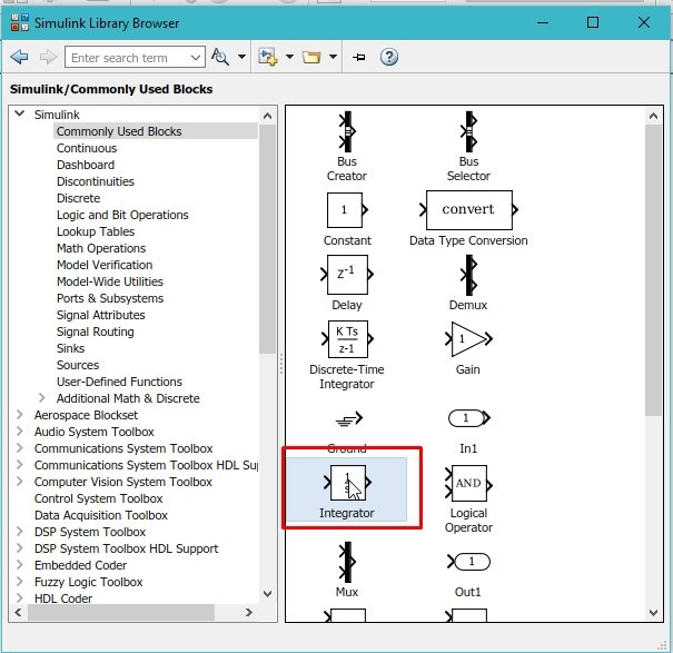
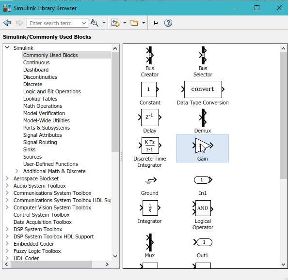
In the Simulink Library Browser, a large number of blocks are present. Click on the most commonly used subsection, as we can see in the following figure.

Differential Equation

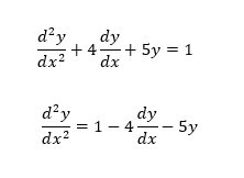
We will write a Simulink program, or, in simple words, we will create a block diagram that will solve the differential equation. The first step we need to take here is to rearrange the differential equation. On the left-hand side, write the highest-order derivative, and move all the remaining terms to the right-hand side. Refer to the figure below.

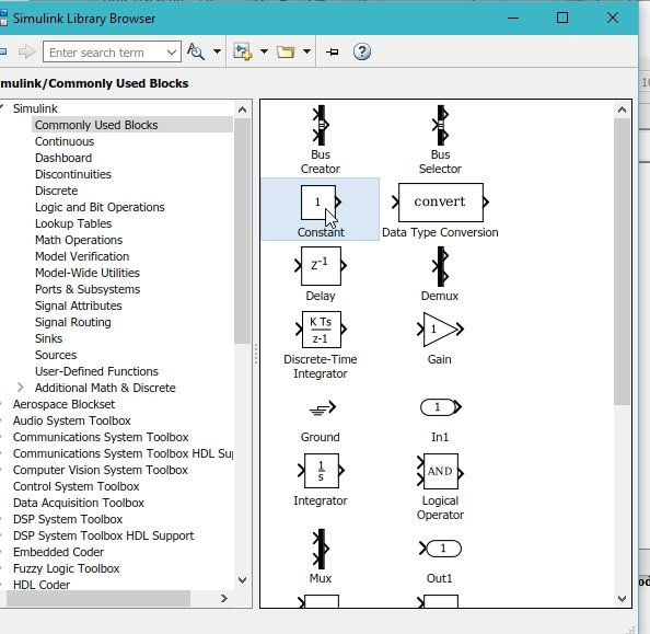
From the library browser, select the commonly used blocks and then select the integral block, as shown in the figure below.

Order of Integral

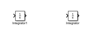
Drag and drop the integral block on the Simulink blank project created previously. Also save the project so we can use it later, as we have done in previous tutorials. If we are working with a second-order differential equation, we will place two integral blocks as in the following figure.

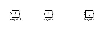
And if we are working with a third-order differential equation, we will be using three integral blocks. We can see this in the figure below.

Placing Components

In our case, however, the number of blocks to be used is 2, as the order of the differential equation is 2. To provide the co-efficient present in the equation, i.e., we will use gain blocks as shown in the figure below.

We will need two gain blocks: one with a gain of 4 and another with a gain of 5. Also, to place the 1 present on the right hand side of the given equation, we will need a constant block, as shown in the figure below.

To add all the terms on the right-hand side of the equation, we will use a summation block, as shown in the figure below.

Place all the components as shown in the figure below, before jumping to the connecting portion.

Flipping Block

As we want to first multiply the term and then add it, we should flip the gain block. This can be done by right-clicking on the block, selecting Rotate & Flip, and then selecting Flip Block, as shown in the figure below.

Double-click on the gain block and change the gain of the block to value 4 as shown in the figure below.

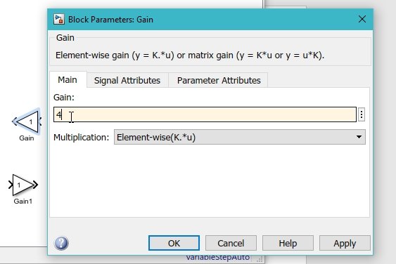
Do the same with the other gain block and change its gain to 5, as shown in the figure below.

Next comes the summation block. Double-click on the summation block. We can also change the shape of the summation block from round to rectangle in the block parameters dialog box, as shown in the figure below.

We can also change the number of terms to be added here by changing the sequence of the list of signs in the parameters of the block, and we can also change them from sum to subtract, as shown in the figure below.

Wire Connections

This list is adjusted according to the right-hand side of the rearranged equation. Connect the constant to the + side of the sum block as shown in the figure below.

Now, connect all the integration blocks together and label them accordingly to perform all the derivative iterations as shown in the figure below.

After this, connect the wire with the gain block labeled as 4 and connect the output of the gain block to the negative sign of the sum block, as shown in the figure below.

Let’s now evaluate the third term, i.e., connect the wire labeled yto the input of the gain block with gain 5 and connect its output to the only left slot in the sum block as shown in the figure below.

From the library browser, select an oscilloscope from the commonly used blocks named Scope,as shown in the figure below.

Simulink Model

Connect it at the output, i.e., attach it to the end of the wire labeled y. The complete block diagram to perform the solution of the differential equation is shown in the figure below.

Run the block diagram from the Run icon, as shown in the figure below.

Simulation

After the simulation is complete, double-click on the scope, and the waveform of the equation will be displayed as shown in the figure below.

Exercise:

• Perform the above-mentioned problem on a third order differential equation. Use the equation given below and solve it in Simulink.

Conclusion

In conclusion, this tutorial provides an in-depth overview of solving differential equations using Simulink. It covers step-by-step procedures along with an explanation of an example to help us better understand the concept. You can utilize this to design and solve more complex differential equations using the integrator in Simulink. At last, we have provided an exercise to reinforce the concept of this tutorial. Hopefully, this tutorial was helpful in expanding your knowledge in regards to Simulink.

You may also like to read:

• ESP32 Send Emails Through SMTP Server (Plain text, HTML, and Attachments)
• Raspberry Pi Pico W MQTT Client Publish Subscribe Messages
• Direct Memory Access (DMA) Introduction
• Getting started with Keil uVision: Write your first Program for Tiva LaunchPad
• UCC25600 High-Performance Resonant Mode Controller
• MAX7219 LED Dot Matrix Display Interfacing with Arduino

This concludes today’s article. If you face any issues or difficulties, let us know in the comment section below.