Least Laxity First (LLF) is a job level dynamic priority scheduling algorithm. It means that every instant is a scheduling event because laxity of each task changes on every instant of time. A task which has least laxity at an instant, it will have higher priority than others at this instant.
LLF is an optimal algorithm because if a task set will pass utilization test then it is surely schedulable by LLF. Another advantage of LLF is that it some advance knowledge about which task going to miss its deadline. On other hand it also has some disadvantages as well one is its enormous computation demand as each time instant is a scheduling event. It gives poor performance when more than one task has least laxity.
Least Laxity First (LLF) Scheduling Algorithm Introduction
Least Laxity First (LLF) is a scheduling algorithm used in real-time systems to determine the order in which to execute tasks or jobs. The main goal of the LLF algorithm is to minimize the laxity (the amount of time a task can be delayed without missing its deadline) of each task. Tasks with the least laxity are given priority and are scheduled to run next.
LLF Basic Steps
Here are the basic steps of the Least Laxity First (LLF) scheduling algorithm:
Initialize Laxity: Calculate the initial laxity for each task. Laxity is defined as the difference between the absolute deadline and the remaining execution time.

Find the Task with the Least Laxity: Identify the task with the smallest laxity value. This task has the highest priority because it is closest to missing its deadline.
Execute the Selected Task: Schedule and execute the task with the least laxity. Update the remaining execution time for this task.
Update Laxity for Other Tasks: Recalculate the laxity for all other tasks in the system based on the time that has passed and the remaining execution time.
Repeat: Continue this process, selecting and executing tasks with the least laxity until all tasks have been completed.
More formally, priority of a task is inversely proportional to its run time laxity. As the laxity of a task is defined as its urgency to execute. Mathematically it is described as

Here di is the deadline of a task, Ci is the worst-case execution time(WCET) and Li is laxity of a task. It means laxity is the time remaining after completing the WCET before the deadline arrives. For finding the laxity of a task in run time current instant of time also included in the above formula.
Here is the current instant of time and is the remaining WCET of the task. By using the above equation laxity of each task is calculated at every instant of time, then the priority is assigned. One important thing to note is that laxity of a running task does not changes it remains same whereas the laxity all other tasks is decreased by one after every one-time unit.
Example of Least Laxity First Scheduling Algorithm
An example of LLF is given below for a task set.
The table shows an example task set and the corresponding values for release time (ri), execution time (Ci), deadline (Di), and period (Ti) for each task. Here is a breakdown of each column in the table:
- Task: This column represents the name or identifier of each task in the task set. In the given example, the tasks are labeled as T1, T2, and T3.
- Release time (ri): This column indicates the time at which each task becomes available or ready for execution. The release time can be thought of as the starting point for each task’s execution. In the example, all tasks are released at time t=0.
- Execution time (Ci): This column specifies the amount of time required to complete the execution of each task. It represents the worst-case execution time (WCET) for the tasks. For example, task T1 requires 2 time units to complete its execution.
- Deadline (Di): This column represents the absolute deadline by which each task must complete its execution. The deadline indicates the maximum allowable time between the task’s release and its completion. In the example, task T1 has a deadline of 6 time units.
- Period (Ti): This column denotes the time interval between consecutive releases of each periodic task. Periodic tasks are tasks that repeat at regular intervals. In the example, all tasks have the same period of time, with a value of 6, 8, and 10 time units for tasks T1, T2, and T3, respectively.
| Task | Release time(ri) | Execution Time(Ci) | Deadline (Di) | Period(Ti) | |
| T1 | 0 | 2 | 6 | 6 | |
| T2 | 0 | 2 | 8 | 8 | |
| T3 | 0 | 3 | 10 | 10 | |
Example Time Diagram
By considering these values, the Least Laxity First (LLF) scheduling algorithm can determine the order in which to execute the tasks based on their laxity (the amount of time a task can be delayed without missing its deadline). Tasks with the least laxity are given priority and scheduled to run next.
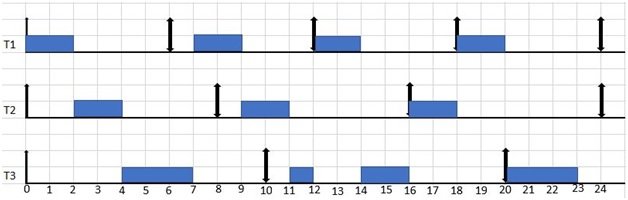
Figure 4. LLF scheduling algorithm
Explanation
- At t=0 laxities of each task are calculated by using equation 4.2. as
L1 = 6-(0+2) =4
L2 = 8-(0+2) =6
L3= 10-(0+3) =7
As task T1 has least laxity so it will execute with higher priority. Similarly, At t=1 its priority is calculated it is 4 and T2 has 5 and T3 has 6, so again due to least laxity T1 continue to execute.
- At t=2 T1is out of the system so Now we compare the laxities of T2 and T3 as following
L2= 8-(2+2) =4
L3= 10-(2+3) =5
Clearly T2 starts execution due to less laxity than T3. At t=3 T2 has laxity 4 and T3 also has laxity 4, so ties are broken randomly so we continue to execute T2. At t=4 no task is remained in the system except T3 so it executes till t=6. At t=6 T1 comes in the system so laxities are calculated again
L1 = 6-(0+2) =4
L3= 10-(6+1) =3
So T3 continues its execution.
- At t=8 T2 comes in the system where as T1 is running task. So at this instant laxities are calculated
L1 = 12-(8+1) =3
L2= 16-(8+2) =6
So T1 completes its execution. After that T2 starts running and at t=10 due to laxity comparison T2 has higher priority than T3 so it completes it execution.
L2= 16-(10+1) =5
L3= 20-(10+3) =7
t=11 only T3 in the system so it starts its execution.
- At t=12 T1 comes in the system and due to laxity comparison at t=12 T1 wins the priority and starts its execution by preempting T3. T1 completes it execution and after that at t=14 due to alone task T3 starts running its remaining part. So, in this way this task set executes under LLF algorithm.
Enhanced Least Laxity First Scheduling Algorithm
LLF is good for avoiding transient overload and domino effect occurring in EDF. But it also has a shortcoming, that is thrashing. When more than one task has least laxity than this phenomenon of Thrashing occurs. Thrashing is the behavior of preemption by the tasks one another at each time tick. This kind of preemption results in context switch at each instant of time. This context switching results in more computation power consumption as switching from one task to another which result in saving and loading registers, memory mapping and updating many tables and lists. So, it results in loss of computation time as well.
To overcome this short come of LLF an improved version of LLF is introduced that is Enhanced least laxity first scheduling algorithm (ELLF). IN ELLF whenever more than one task has least laxity than they all are grouped together and EDF is applied within the group whereas taking this group as a single task LLF is applied to this group and other remaining tasks in the task set.
An example of LLF with thrashing is given below
| Task | Release time(ri) | Execution Time(Ci) | Deadline (Di) | Period(Ti) | |
| T1 | 0 | 3 | 12 | 7 | |
| T2 | 0 | 4 | 13 | 10 | |
| T3 | 0 | 5 | 14 | 12 | |
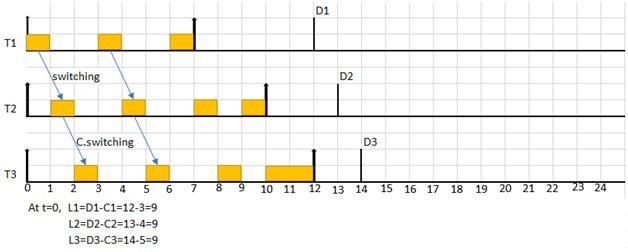
So, to overcome this context switching due to thrashing We employ ELLF on the same example by grouping together the tasks having same least laxity, then apply EDF to avoid context switching.

Conclusion
In conclusion, the Least Laxity First (LLF) scheduling algorithm is a dynamic priority scheduling algorithm used in real-time systems. Its main objective is to minimize the laxity of each task, which represents the amount of time a task can be delayed without missing its deadline. By assigning priority based on the task’s laxity, LLF ensures that tasks with the least laxity are given higher priority and scheduled to run next.
LLF is considered an optimal algorithm as it guarantees schedulability for task sets that pass the utilization test. However, LLF can suffer from thrashing when multiple tasks have the same least laxity, resulting in frequent context switching. To address this issue, an enhanced version called Enhanced Least Laxity First (ELLF) scheduling algorithm can be used, which groups tasks with the same least laxity and applies Earliest Deadline First (EDF) scheduling within the group. Overall, LLF and its enhanced version, ELLF, provide effective scheduling solutions for real-time systems.
You may also like to read:
Hi there. thank you for your efforts in making an example about LLF algorithm, but I have two questions about the LLF example. 1st: at t=6 why you calculated L1 with t=0?. 2nd: if we applied what happens in my 1st question on T1 again in t=12 that means L1=12-(0+2) =10 and then L3=20-(12+2)=6 and in this case T3 will have the least laxity than T1, so T3 should be start its execution, am I right?
I hope to give me an efficient answer please.
Thanks again.
second answer: L1=12-(6+2) =4; Four is a correct as in a tutorial.
how T1, At t=1 its priority is calculated it is 4