In this tutorial, we will explain the workings of lags and delays in Simulink. Lags and delays seem to be similar terms, but in fact they are not. In this tutorial, we will discuss the particular difference between lags and delays. In Simulink, there are multiple blocks that can perform the delay operation with a little distinction in their functionality. We will also discuss this distinction in this tutorial, along with the workings and implementation of each block. We will provide a comprehensive example regarding the workings of delay. Here we will discuss two types from the Simulink library browser, i.e., Delay Block and Transport Delay Block. Finally, we will also explain the workings of lags in the output or response of a system and their differences.
Introduction to Lags and Delay in Simulink
Lags and delays play a vital role in representing and simulating systems in Simulink. First, let’s see what the difference is between lag and delay. The delay is the extra time taken by the system to execute the output when we require it. Whereas the lag is an immediate response at output while the complete output is spread over time, resulting in a change of shape.
In Simulink, we can use delay blocks to add delay to our system. The setting of the delay block is done by setting its parameter according to our requirements. Now, for adding lags in Simulink, we can use the Transport Delay block. In the case of a unit step function, this will provide us with a slope instead of a normal straight line when the step function changes from 0 to 1. This way, we can add delays and lags to our Simulink model.
How to Use Lags and Delay in Simulink
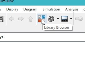
Open MATLAB and then Simulink, as we have been doing in previous tutorials. Now create a new blank model in Simulink and save it so we can use it in the future. In the blank model, click on the library browser icon, as we can see in the figure below.
Now, first of all, we want a source on which we will apply delay and see lags; therefore, in the library browser, click on the sources block, and we will select a source. Refer to the figure below.

Placing Components
From the sources section of the library block, select the step block. At the output of this block, we will receive a step input. Refer to the figure below.

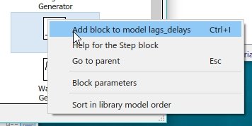
This block will be used as input, and we will apply delays or lags to this input waveform, as we will see shortly. Right-click on this block and click on Add block to the model to add the block to the model we created previously, as we can see in the figure below.
Now we also need a sink or an output block at which we will see the delayed and lagged output. Therefore, from the library browser, select the sinks section as shown in the figure below.
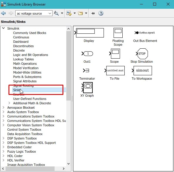
From this section, select the block named scope, as we have been using it in all the previous tutorials. Add the block to the model as we have done previously.

Now double-click on the step block, and from the block parameters dialog box, change the step time of the step input to 2, as shown in the figure below, so that the input and all the delayed blocks are visible at the oscilloscope output.

Simulink Model
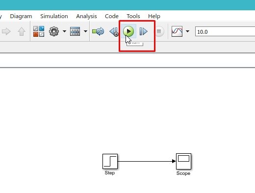
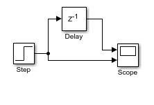
Connect the step block to the scope block, as shown in the figure below.

Simulation
Run the blocks from the run button, as shown in the figure below.
After running the block, double-click on the scope to see the output, and the output of the step is shown in the figure below.

Delay Block
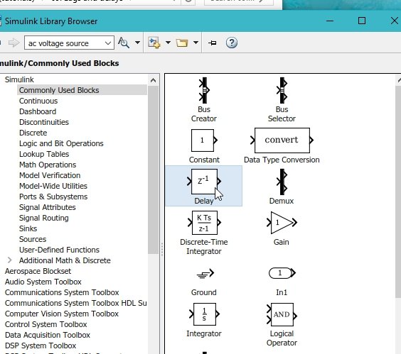
Now let’s apply the delay function to the input step. For that purpose, open the commonly used blocks section of the library browser and select the delay block, as shown in the figure below.
As we are interested in viewing both the input and the delayed input in the same window, we will increase the number of input ports from 1 to 2. We can do this by simply right-clicking on the delay block and then clicking on the signals and ports label. After this, we click on the number of input ports and then on 2, as shown in the figure below. This will change the number of ports in the scope block to two.

Simulink Model with Delay
Connect the simple input to one input port of the scope block and the delayed input to the other, as shown in the figure below.
Simulation
Run the blocks and again open the scope window by double-clicking on the scope block. The normal input and the delayed input are shown in the figure below.

We can also change the delayed time of the block by double-clicking on the delay block and changing the value parameter in the delay block. The delayed output with a different delay time is shown in the figure below.

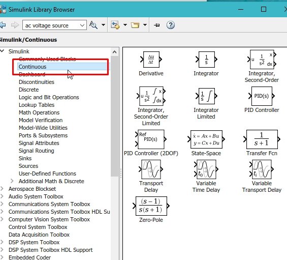
Now let’s see the functionality of a different delay block in Simulink. From the library browser, select the continuous section, as we can see in the figure below.
Transport Delay Block
From the continuous block of the library browser, select the block named transport delay, as shown in the figure below.

Add the block to the model, and after that, double-click on the block, and from the block parameters, we can change the delay time of the block. For example, we set the delay time to 5 seconds here. Refer to the figure below.

Now that we have three different inputs to display on the oscilloscope, we need to change the number of input ports on the oscilloscope to three, as we have done previously, as shown in the figure below.

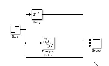
Simulink Model with Transport Delay Block
Connect the newly created delayed output to the third input port of the scope, as shown in the figure below.
Simulation
The input of the step and the two delayed inputs as the outputs are displayed simultaneously on the same graph in the scope when you run the block diagram, as shown in the figure below.

Transfer Function Block
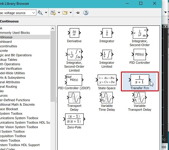
The red wave in the above graph is the input of the step block, the yellow is the output of the delay block, and the blue is the output of the transport delay block. The difference in the outputs of the delayed blocks is visible from the graphs shown in the figure above. The small slope of the transport delay blocks’ output is also referred to as a lag, which occurs in all the physical circuits of real time. Let’s discuss this lag operation further using another block. From the continuous section of the library browser, select the transfer function block as shown in the figure below.
Simulink with Transfer Function
Place that transfer function block in the model, and at the input of it, connect the step input, and at the output, connect the scope. But first, we must change the number of input ports in the scope, as we have done previously. The connected diagram is shown in the figure below.

Now run the block diagram and double-click on the scope block to see the output. As there are multiple outputs, it might be difficult for you to recognize which output is who’s. Therefore, from the scope window, click on the view label at the top, and a drop-down will appear. From that drop-down, check the label named legends, as shown in the figure below.

These legends will assign proper names to each waveform, as shown in the figure below.

The lagged output is the red one and is the same as the input, but it is showing the real-time effect of the normal step input function.
Conclusion
In conclusion, this provides an in-depth overview of implementing lags and delays in Simulink block diagrams. It covers step-by-step procedures along with an explanation of an example to help us better understand the concept. You can utilize this concept to add lag or delays to your projects. Hopefully, this was helpful in expanding your knowledge of Simulink.
You may also like to read
- ESP8266 NodeMCU Erase Flash Memory Perform Factory Reset
- ESP32 ESP8266 SMTP Client Send Sensor Readings via Email using MicroPython
- How to Use Loops in Simulink: Tutorial 7
- UART Communication with Pic Microcontroller( Programming in MPLAB XC8 )
- BME680 with ESP32 using Arduino IDE (Gas, Pressure, Temperature, Humidity)
- ATMega32 Microcontroller
This concludes today’s article. If you face any issues or difficulties, let us know in the comment section below.