In this tutorial, we will explain the workings of a rectifier. Rectifiers are one of the most basic circuits in electronics. At the start, we provide a comprehensive introduction to rectifiers, along with their types, uses, and the effect of the type of rectifier on the output. After that, we implement the rectifier circuit in MATLAB’s Simulink. We will also discuss the difference between both types of rectifiers and compare the output of the block diagram constructed on Simulink.
Introduction to Rectifier
In electrical engineering, the rectifier is one of the most simple circuits. The basic purpose of a rectifier is to convert alternating current (AC) to direct current (DC). For beginners, the definition of AC voltage can be taken as the voltage that changes its direction from positive voltage to negative voltage across the same terminal in a specified period of time over and over again. A simple sinusoidal wave is an AC wave. However, DC can be defined as a constant source of voltage that remains either positive or negative over time.
Types of Rectifiers
We can classify rectifiers into two major types:
- Half wave rectifier
- Full wave rectifier
Half Wave Rectifier
A half wave rectifier only rectifies (converts to DC) the positive part of the AC voltage and skips the negative part. This rectifier is rarely used in common practice because of the loss of power due to the wastage of the negative part.
Full Wave Rectifier
A full wave rectifier, however, uses both the positive and negative parts of the AC wave to rectify. It will pass the positive wave as it is and will invert the negative part of the wave to appear positive on the load with the help of a bridge, as we will see shortly. Along with some filters to remove ripples, we can get a perfect DC wave at the output. Due to less power loss and a closer resemblance to DC, this circuit is used more frequently compared to the former one.
Full Wave Rectifier Simulation in Simulink
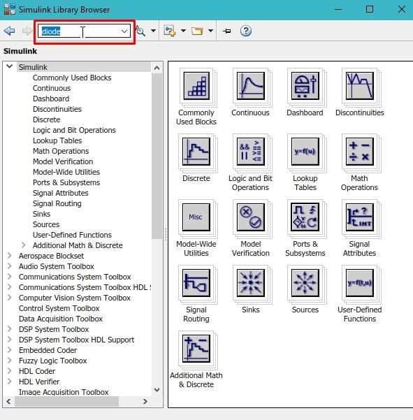
Open MATLAB and then open Simulink using the Simulink icon on MATLAB, as we have been doing in previous tutorials. Create a new blank model and save it first so we can access it in the future. Now, click on the library browser icon on the recently created Simulink model. And in the library browser’s search bar, type “diode”, as we can see in the figure below. Remember that diodes are the main component in any type of rectifier, and here we are going to design a full wave rectifier. As the half wave rectifier is simpler, we will leave it to you for practice purposes.
From the list of diodes, select the most suitable diode. We prefer to select the one with protection, as shown in the figure below.

Full Wave Rectifier Bridge
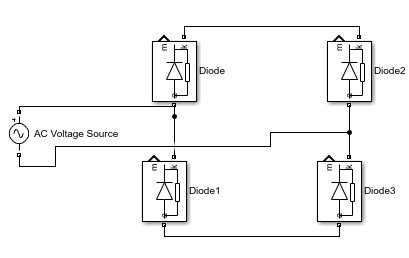
Place four such diodes. Those who are familiar with rectifiers must know that in a full wave rectifier, there is a bridge of diodes. This bridge is made up of four diodes; hence, place four such diodes. Place two pairs of diodes in series, then connect these two pairs in parallel as shown in the figure below.

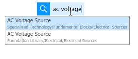
Now, click anywhere on the screen, and from the search box, search for the AC voltage source as we have done previously, as shown in the figure below.
Connect the positive side of the AC source between the two serially connected diodes and the negative side to other serially connected diodes, as shown in the figure below.
After the source is connected, we also need a ground to complete the circuit. We will search for it, as shown in the figure below.

Placing and Configuring RLC branch
Connect the ground to the bottom of the circuit. Now, from the search bar, search for the series RLC branch. Refer to the figure below.

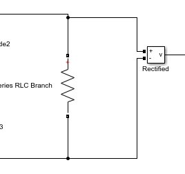
Now, we add the RLC block to the model. After this, double-click on the RLC branch, and from the parameters block, select the resistor branch only, as shown in the figure below.

Connect this resistor branch to the load of the bridge rectifier, and the diagram with the load connected will look like the one shown in the figure below.

Now we need to set the input parameters of the AC voltage source. Double-click on the input voltage source and set the peak amplitude of the voltage to 10 V, as shown in the figure below.

Now, if we run this block diagram, we will encounter an error for the requirement of a power GUI. Power GUI is a block that is essential in Simulink to run an electronic circuit. In the search bar, search “powergui”, as shown in the figure below.

Setting Voltmeter
Next, we need a voltage measuring device in order to see the voltage waveform at the output. Again, in the search bar, write voltage measurement, as shown in the figure below.

Place two such voltmeters on the model. Connect one of the voltmeters across the load resistor, as we are basically interested in measuring and viewing the voltage waveform at the load resistor. Refer to the figure to see how to connect the voltmeter to the load.
Also, we need a reference waveform to compare the output at the load with. Therefore, we will also measure the voltage at the input by connecting a voltmeter across the input AC source, as shown in the figure below.

Now, we need to see the waveform at the load and the input to visualize what actually happens in a rectifier. To visualize a waveform, we need to use an oscilloscope. In the search bar’s search scope, as shown in the figure below.

Simulink Model
Place the block on the model near the load. We want to view two waveforms, one of the input and the other of the output. Therefore, we need two input ports in scope. Change the number of input ports in the scope to two, as we have done in previous tutorials (refer to the RLC tutorial). At the two input ports, connect the input voltmeter and the output load voltmeter, as shown in the figure below.

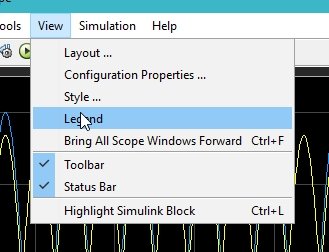
Run the model by pressing the run button and then double-clicking on the scope. We want to see the legends on the waveform displayed by scope; hence, click on the view button and check the legends label as shown in the figure below.
Simulation
The rectified output at the load and the input AC are both shown in the figure below.

The output is a pulsating DC. It can be converted to plain DC by using filters and regulators.
Exercise
- Perform the analysis on a half wave rectifier using MATLAB’s Simulink. It would be much simpler than the one performed in this tutorial.
(Hint: Number of diodes to be used will be one.)
Conclusion
In conclusion, this tutorial provides an in-depth overview of designing and simulating a full wave rectifier in Simulink. It covers step-by-step procedures along with explanations of an example to help us better understand the concept. You can utilize this concept to design and simulate a half wave rectifier as well. At the end, we provide an exercise to reinforce the concept of this tutorial. Hopefully, this was helpful in expanding your knowledge of Simulink.
You may also like to read:
- High Pass Filter Simulation using PSpice: Tutorial 14
- ESP32 Send Sensor Readings to ThingSpeak using Arduino IDE (BME280)
- DC Motor Interfacing with Atmega32 and L293
- Interface GT511C3 Fingerprint Scanner Module with Arduino
- 28BYJ-48 Stepper Motor with Raspberry Pi Pico using MicroPython
- INTRODUCTION TO ARDUINO ETHERNET SHIELD
- Control Relay Module Remotely with ESP32 Web Server and 220V Lamp
This concludes today’s article. If you face any issues or difficulties, let us know in the comment section below.