In this tutorial, we will explain the workings of controlled rectifiers and how we can implement them using MATLAB Simulink. Rectifiers are one of the very basic circuits of electronics; however, controlled rectifiers are those whose output waveform can be controlled using electronic switches by controlling their firing angles. At the start, we will provide a comprehensive introduction to controlled rectifiers, along with their types and uses. After that, the circuit of controlled rectifiers is implemented in MATLAB’s Simulink. At the end, we have provided an exercise for you to perform on your own regarding the concepts discussed in the tutorial.
Introduction to Rectifiers
Controlled rectifiers are the basic components of power electronics. As the name suggests, in a controlled rectifier, we can control the shape of the output waveform of the rectifier with the help of switches. The waveform shape will depend on the firing angle of the switch connected to the bridge.
Types of rectifiers
Controlled rectifiers can be classified into two major types:
- Half wave rectifier
- Full wave rectifier
Half wave rectifier
Unlike simple half wave rectifiers, half wave and full wave controlled rectifiers depend on the number of switches used in the circuit. The pulses given to the switches have a specified Pulse Width Modulation (PWM), and that PWM will decide the shape of the rectified output wave. The PWM of the pulse is also used to define the firing angle of the rectifier, as we will see shortly.
Full wave rectifier
A full wave rectifier, however, uses both the positive and negative parts of the AC wave to rectify. Again, in this case, we use switches with gate pulses for the firing angles of the rectified output. The rectified output will not be a pure sinusoidal waveform, although it will be a distorted sine 0 output before sinusoidal and rectified sine waves after the firing angle of the pulses in the gate input of switches.
Controlled Rectifiers in Simulink
In the model, we are going to discuss how to design a half wave controlled rectifier, and we will leave the design of a full wave controlled rectifier as an exercise for you.
Open MATLAB to create a model, and then open Simulink by clicking on the icon present on the main page of MATLAB or by typing simulink in the command window of MATLAB. Once the Simulink window pops up, click on the block named blank model, as we have been doing in the previous tutorials. After that, open the library browser, and in the search bar of the library browser, search “Pulse generator”, as shown in the figure below, and press enter.

After searching, the only block in the search result will be the source “pulse generator”, as shown in the figure.

Add Block to Model
Drag and drop this block on the Simulink model, or add it to the Simulink model by right-clicking on it and selecting Add to Model. Refer to the figure below.

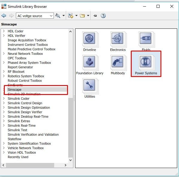
Let’s first add all the sources to the model, and after that, we will move on to the main components. The power to the rectifier will be provided by the AC voltage source. Let’s now locate the position of the AC voltage source in the library browser. In the library browser, select the Simscape submenu and then select Power System from its components, as we can see in the figure below.
In the power system block, select the block named Specialized Technology, as shown in the figure below.

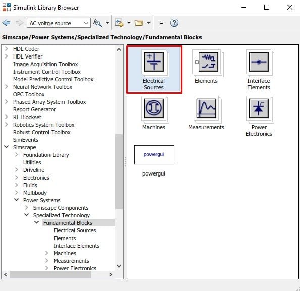
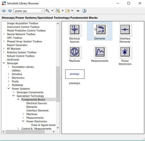
From this block, select the fundamental blocks as shown in the figure below.

Sources
From the Fundamental Blocks submenu, select the Electrical Sources block.
This is the place where all the power sources reside; select an AC voltage source from inside that block as shown in the figure below.

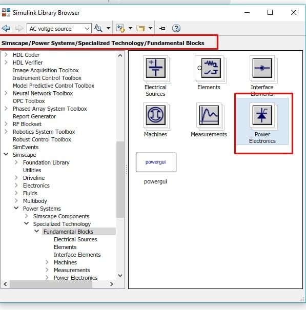
Here we will use the Add Block to Model option to add this block to our model. Now go back to the fundamental block model we encountered on our way here, and from that block, select the block named power electronics, as shown in the figure below.
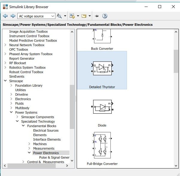
From this block, select the block of thyristors (used in place of diodes in controlled rectifiers) and add the block to the model as shown in the figure below.
Go back to the fundamental block and select the power GUI, as shown in the figure below, and add it to the model. The purpose of this block is to provide a kind of source code for the blocks used in the power section.

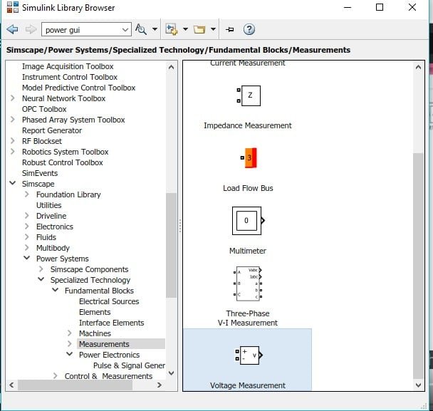
Again, from the fundamental blocks, select the measurement block, as shown in the figure below.

Voltage Measurement Block
From this block, select the Voltage Measurement block and place two such blocks on the model, one for input measurement and one for output, as shown in the figure below.
Again, go back to the fundamental blocks and select the Elements block (for placing loads), as shown in the figure below.
From this block, select the series RLC branch, so we can test our circuit for any kind of load, and place it on the model as shown in the figure below.

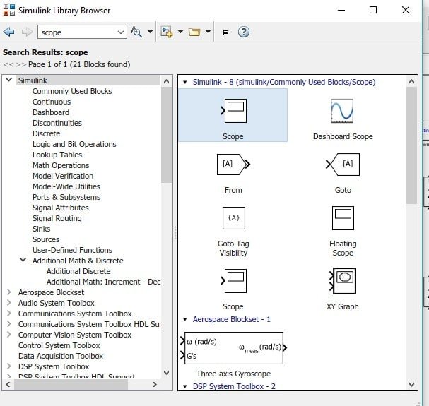
The last thing we need to place is the scope, so we can see the waveform of the rectifier at the output. Search scope in the search bar of the library browser and add it to the model as shown in the figure below.
Place Component
Now that we are done with placing components, let’s move toward the model and place the components accordingly, as shown in the figure below.
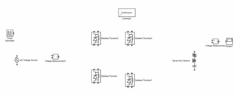
Connect the thyristors in the form of a bridge for full wave rectification, as shown in the figure below.
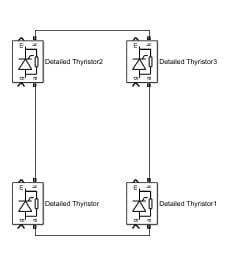
Connect the power source in the same fashion as we have done in the case of a simple full wave rectifier, and also connect the load. Now connect the pulse generator to the input pin g of the thyristor and also connect voltage measuring blocks at the input and output as shown in the figure below.

At the output, connect the scope, but first we need to make some changes. Double-click on scope, then select file, and change the number of input ports to 2. Refer to the figure below.

Simulink Model
To the input ports of the scope, connect the input and output of the controlled rectifier as shown in the complete block diagram below. Also, double-click on the RLC branch and change it to only resistors and set its value to 400.

Parameters
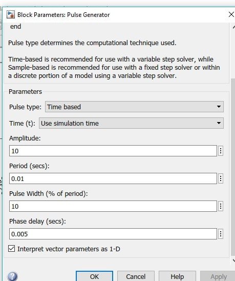
Now set the parameters of the pulse generator as shown in the figure below.
Also, we have to change the parameters on the input AC voltage source, as shown in the figure below.

Change the layout of the scope to two blocks by changing the properties of the scope as shown below.


Simulation
Now run the model using the run button and adjust the scale of the scope. The output of the full wave controlled rectifier is shown in the figure below.

We can change the angle of control by changing the phase delay in the pulse generator parameter.
Exercise
- Perform the analysis on a full wave controlled rectifier using MATLAB’s Simulink. It would be much simpler than the one performed in this tutorial.
(Hint: Number of diodes to be used will be two.)
Conclusion
In conclusion, this article provides an in-depth overview of designing and simulating a controlled rectifier in Simulink. It covers step-by-step procedures along with an explanation of an example to help us better understand the concept. You can utilize this concept to design more advanced and complex rectifiers. At the end, we provided an exercise to reinforce the concept of this tutorial. Hopefully, this was helpful in expanding your knowledge of Simulink.
You may also like to read:
- Control ESP32 Outputs using Google Assistant and Adafruit IO
- BME680 with ESP32 using Arduino IDE (Gas, Pressure, Temperature, Humidity)
- MicroSD Card Module with STM32 Blue Pill using STM32CubeIDE
- DC Motor Control with LabVIEW and Arduino – Tutorial 3
- ESP32-CAM Take Photo and Save to MicroSD Card with Timestamp Date and Time
- FreeRTOS Software Timers with Arduino – Create One-shot and Auto-Reload Timer
This concludes today’s article. If you face any issues or difficulties, let us know in the comment section below.
How can view output vtg value